Rankine–Hugoniot conditions

The Rankine–Hugoniot conditions, also referred to as Rankine–Hugoniot jump conditions or Rankine–Hugoniot relations, relate to the behaviour of shock waves traveling normal to the prevailing flow. They are named in recognition of the work carried out by Scottish engineer and physicist William John Macquorn Rankine^[1] and French engineer Pierre Henri Hugoniot.^[2] See also Salas (2006)^[3] for some historical background.

1 Introduction
2 The jump condition
3 Euler equations shock condition
4 Stationary shock
5 See also
6 References

Introduction

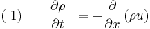
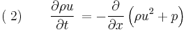
Consider a one-dimensional, calorically ideal gas described by a polytropic equation-of-state and operating under adiabatic conditions. In addition, assume that the fluid is inviscid (negligible viscosity effects). Such a system can be described by the following system of conservation laws, known as the 1D Euler equations

$(\;1)\quad \quad\frac{\partial\rho}{\partial t} \;\; = -\frac{\partial}{\partial x}\left(\rho u\right)$

$(\;2)\quad \quad\frac{\partial\rho u}{\partial t} \, = -\frac{\partial}{\partial x}\left(\rho u^{2}%2Bp\right)$

$(\;3)\quad \quad\frac{\partial\rho E}{\partial t} = -\frac{\partial}{\partial x}\left[\rho u\left(e%2B\frac{1}{2}u^{2}%2Bp/\rho\right)\right],$

where,

$\rho = \,$ fluid mass density, [kg/m³]

$u = \,$ fluid velocity, [m/s]

$e = \,$ fluid-specific internal energy, [J/kg]

$p = \,$ fluid pressure, [Pa]

$t = \,$ time, [s]

$x = \,$ distance, [m], and

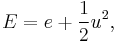$E = e%2B\frac{1}{2}u^{2},$ fluid-specific total energy, [J/kg].

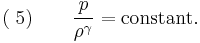
For adiabatic conditions a polytropic process can be represented by the equation-of-state,

$(\;4)\quad\quad p=\left(\gamma-1\right)\rho e,$

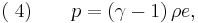
where $\gamma$ represents the polytropic exponent (equal to the ratio of specific heats $c_p/c_v\,$ ) of the polytropic process

$(\;5)\quad \quad \frac{p}{\rho^\gamma} = \text{constant}.$

For an extensive list of compressible flow equations, etc., refer to NACA Report 1135 (1953).^[4]

Note: For a calorically ideal gas $\gamma \,$ is a constant and for a thermally ideal gas $\gamma \,$ is a function of temperature.

The jump condition

Before proceeding further it is necessary to introduce the concept of a jump condition – a condition that holds at a discontinuity or abrupt change.

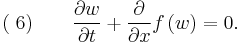
Consider a 1D situation where there is a jump in the scalar conserved physical quantity $w$ , which is governed by the hyperbolic conservation law

$(\;6) \quad\quad \frac{\partial w}{\partial t}%2B\frac{\partial}{\partial x}f\left(w\right)=0.$

Let the solution exhibit a jump (or shock) at $x=x_{s}(t)$ and integrate over the partial domain, $x\in\left(x_{1},x_{2}\right)$ , where $x_{1}<x_{s}(t)$ and $x_{s}(t)<x_{2}$ ,

$(\;7) \quad\quad \frac{d}{dt}\left(\int_{x_1}^{x_s(t)}w \, dx %2B \int_{x_s(t)}^{x_2} w\,dx\right) = -\int_{x_1}^{x_2}\frac{\partial}{\partial x}f\left(w\right)\,dx$

$(\;8) \quad\quad \therefore w_1\frac{dx_s}{dt}-w_2 \frac{dx_s}{dt} %2B \int_{x_1}^{x_s(t)} w_t \, dx %2B \int_{x_s(t)}^{x_2}w_t \, dx = -\left.f\left(w\right)\right|_{x_1}^{x_2}$

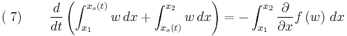
The subscripts 1 and 2 indicate conditions just upstream and just downstream of the jump respectively. Note, to arrive at equation (8) we have used the fact that $dx_1/dt=0$ and $dx_2/dt=0$ .

Now, let $x_1\rightarrow x_s(t)$ and $x_2\rightarrow x_s(t)$ , when we have $\int_{x_1}^{x_s(t)}w_t \, dx\rightarrow 0$ and $\int_{x_s(t)}^{x_2}w_t \, dx\rightarrow0$ , and in the limit

$(\;9) \quad\quad s\left(w_1 - w_2\right) = f \left( w_1 \right) - f \left( w_2 \right),$

where we have defined $s=dx_s(t)/dt \,$ (the system characteristic or shock speed), which by simple division is given by

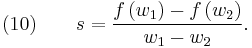
$(10) \quad\quad s = \frac{f\left(w_1\right) - f\left(w_2 \right)}{w_1 - w_2}.$

Equation (9) represents the jump condition for conservation equation (6). A shock situation arises in a system where its characteristics intersect, and under these conditions a requirement for a unique single-valued solution is that the solution should satisfy the admissibility condition or entropy condition. For physically real applications this means that the solution should satisfy the Lax entropy condition

$(11) \quad\quad f^{\prime} \left(w_1\right) > s > f^{\prime} \left( w_2 \right),$

where $f^{\prime}\left(w_1\right)$ and $f^{\prime}\left(w_2\right)$ represent characteristic speeds at upstream and downstream conditions respectively.

Euler equations shock condition

In the case of the hyperbolic conservation equation (6), we have seen that the shock speed can be obtained by simple division. However, for the 1D Euler equations ( 1), ( 2) and ( 3), we have the vector state variable $\left[\rho,\rho u,\rho E\right]^T$ and the jump conditions become

$(12)\quad\quad\quad\quad\; s\left(\rho_2 - \rho_1 \right) = \rho_2 u_2 - \rho_1 u_1$

$(13)\quad\quad\; s\left(\rho_2 u_2 - \rho_1 u_1 \right) = \left( \rho_2 u_2^2 %2Bp_ 2 \right) - \left(\rho_1 u_1^2 %2Bp_1 \right)$

$(14)\quad\quad s\left(\rho_2 E_2 - \rho_1 E_1 \right) = \left[ \rho_ 2 u_ 2 \left( e_ 2 %2B \frac{1}{2} u_2^2 %2Bp_2/\rho_2 \right)\right] - \left[\rho_1 u_1 \left( e_1 %2B \frac{1}{2} u_1^2 %2B p_1/\rho_1 \right)\right].$

Equations (12), (13) and (14) are known as the Rankine–Hugoniot conditions for the Euler equations and are derived by enforcing the conservation laws in integral form over a control volume that includes the shock. For this situation $s$ cannot be obtained by simple division. However, it can be shown by transforming the problem to a moving co-ordinate system, i.e. $v=s-u$ , and some algebraic manipulation, that the shock speed is given by

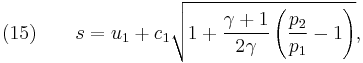
$(15)\quad\quad s = u_1 %2B c_1 \sqrt{1 %2B \frac{\gamma%2B1}{2\gamma} \left( \frac{p_2}{p_1} - 1\right)},$

where 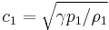$c_{1}=\sqrt{\gamma p_{1}/\rho_{1}}$ is the speed of sound in the fluid at upstream conditions.

See Laney (1998),^[5] LeVeque (2002),^[6] Toro (1999),^[7] Wesseling (2001),^[8] and Whitham (1999)^[9] for further discussion.

Stationary shock

For a stationary shock $s=0$ , and for the 1D Euler equations we have

$(12)\quad\quad\quad\quad\quad\quad\quad\quad\quad\quad\;\; \rho_1 u_1 = \rho_2 u_2$

$(13)\quad\quad\quad\quad\quad\quad\quad\quad\;\; \rho_1 u_1^2 %2B p_1 = \rho_2 u_2^2 %2B p_2$

$(14)\quad\quad \rho_1 u_1 \left( e_1 %2B \frac{1}{2} u_1^2 %2B p_1/\rho_1 \right) = \rho_2 u_2 \left(e_2 %2B \frac{1}{2} u_2^2 %2B p_2/\rho_2 \right).$

In view of equation (12) we can simplify equation (14) to

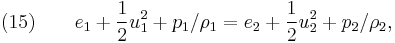
$(15)\quad\quad e_1 %2B \frac{1}{2} u_1^2 %2B p_1/\rho_1 = e_2 %2B \frac{1}{2} u_2^2 %2B p_2/\rho_2,$

which is a statement of Bernoulli's principle, under conditions where gravitational effects can be neglected.

Substituting $u_{1}$ and $u_{2}$ from equations (12) and (13) into equation (15) yields the following relationship:

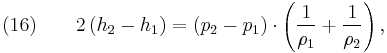
$(16)\quad\quad 2 \left( h_2 - h_1 \right) = \left( p_2 -p_1 \right) \cdot \left(\frac{1}{\rho_1} %2B \frac{1}{\rho_2}\right),$

where $h=\frac{p}{\rho}%2Be$ represents specific enthalpy of the fluid. Eliminating internal energy $e$ in equation (15) by use of the equation-of-state, equation ( 4), yields

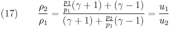
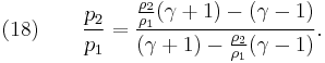
$(17)\quad\quad \frac{\rho_2}{\rho_1} = \frac{\frac{p_2}{p_1} (\gamma%2B1) %2B (\gamma-1)}{(\gamma%2B1) %2B \frac{p_2}{p_1}(\gamma-1)} = \frac{u_1}{u_2}$

$(18)\quad\quad \frac{p_{2}}{p_{1}} = \frac{\frac{\rho_2}{\rho_1} (\gamma%2B1) - (\gamma-1)} {(\gamma%2B1) - \frac{\rho_2}{\rho_1} (\gamma-1)}.$

From physical considerations it is clear that both the upstream and downstream pressures must be positive, and this imposes an upper limit on the density ratio in equations (17) and (18) such that 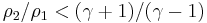$\rho_{2}/\rho_{1}<(\gamma%2B1)/(\gamma-1)\,$ . As the strength of the shock increases, there is a corresponding increase in downstream gas temperature, but the density ratio $\rho_{2}/\rho_{1}$ approaches a finite limit: 4 for an ideal monatomic gas $(\gamma=5/3)$ and 6 for an ideal diatomic gas $(\gamma=1.4)$ . Note: air is comprised predominately of diatomic molecules and therefore at standard conditions $\gamma_{air}\simeq1.4$ .

References

^ Rankine, W. J. M. (1870). "On the thermodynamic theory of waves of finite longitudinal disturbances". Phil. Trans. Roy. Soc. 160: 277. doi:10.1098/rstl.1870.0015. http://gallica.bnf.fr/scripts/get_page.exe?O=55965&E=328&N=11&CD=1&F=PDF.
^ Hugoniot, H. (1887). "Propagation des Mouvements dans les Corps et spécialement dans les Gaz Parfaits" (in French). Journal de l'Ecole Polytechnique 57: 3.
^ Salas, M. D. (2006). "The Curious Events Leading to the Theory of Shock Waves, Invited lecture, 17th Shock Interaction Symposium, Rome, 4–8 September.". http://ntrs.nasa.gov/archive/nasa/casi.ntrs.nasa.gov/20060047586_2006228914.pdf.
^ Ames Research Staff (1953), "Equations, Tables and Charts for Compressible Flow", Report 1135 of the National Advisory Committee for Aeronautics, http://ntrs.nasa.gov/archive/nasa/casi.ntrs.nasa.gov/19930091059_1993091059.pdf
^ Laney, Culbert B. (1998). Computational Gasdynamics. Cambridge University Press. ISBN 978-0521625586.
^ LeVeque, Randall (2002). Finite Volume Methods for Hyperbolic Problems. Cambridge University Press. ISBN 978-0521009249.
^ Toro, E. F. (1999). Riemann Solvers and Numerical Methods for Fluid Dynamics. Springer-Verlag. ISBN 978-3540659662.
^ Wesseling, Pieter (2001). Principles of Computational Fluid Dynamics. Springer-Verlag. ISBN 978-3540678533.
^ Whitham, G. B. (1999). Linear and Nonlinear Waves. Wiley. ISBN 978-0471940906.